Fast Fourier Transform
I have always wanted to learn how the FFT worked. I originally wanted to do this on Rust so I learn the language at the same time learning about the algorithm. However, after implementing the Cooley–Tukey FFT algorithm in the sample size of powers of two in Python. I fell down the rabbit hole of trying to implement the arbitrary size version of the algorithm. I soon discovered the weird world of circular convolution and Bluestein’s algorithm. I ended up just learning about Fourier Transforms rather than Rust. So I will be mostly going through my conceptual understanding of Fourier transforms and implementation of the Fast Fourier transform
Fourier Analysis
Fourier transform/series is so ubiquitous in our world. It’s everywhere from signal processing to the weird and wacky world of physics. But what is it? Well, channel 3blue1Brown explains it better than anything I can come up.1. I might come up with a different blog post to intuitively explain the Fourier transform/series from the perspective of complex analysis. But for now, here is a brief overview.
Fourier Series
Fourier series can be thought up as a way of approximating a periodic function \(f(t) = f(t+T)\) for some \(T\). It involves taking a sum of different sin waves. In general, most well-behaved periodic functions can be decomposed in the following way
\[f(t) = A_{0} +\sum_{n=0}^{\infty} A_{n}\cos\frac{2\pi n t}{T} + B_n\sin\frac{2\pi nt}{T}\]Now using this magical equation \(e^{ix} = \cos x + i\sin x\) the above equation can be expressed as:
\[f(t) = \sum_{-\infty}^{\infty} \widehat{c}_ne^{\frac{2i\pi n t}{T}}\]We can retrieve the \(c_{n}\) from above by using the following arguments
- \[\int_{-\pi}^{\pi} e^{-ix} dx = 0\]
- \[\int_{-\pi}^{\pi} Ce^{-i.0} dx = 2\pi C\]
- \[\int^{D} f(x) + g(x)dx = \int^{D} f(x) dx +\int^{D} g(x)dx\]
We can derive the fact that:
\[\widehat{c}_n = \frac{1}{T}\int_{-\frac{T}{2} }^{\frac{T}{2}} f(t)e^{\frac{-2i\pi n t}{T}} dt\]Fourier Transformation
Now what happens if we do this as we let the period go to infinity? Of course, we have to assume that the sum is well defined from \(\infty\) to \(- \infty\).
Suppose:
\[\omega = \frac{n}{T}\]and
\[\widehat{f}(\omega) = \int_{-\frac{T}{2} }^{\frac{T}{2}} f(t)e^{-2\pi \omega ti} dt\]Then
\[f(t) = \frac{1}{T}\sum_{-\infty}^{\infty} \widehat{f}(\omega)e^{2\pi \omega ti}\]Since \(d\omega = \frac{n+1}{T} - \frac{n}{T} = \frac{1}{T}\)
\[f(t) = \sum_{-\infty}^{\infty} \widehat{f}(\omega)e^{2\pi \omega ti} d\omega\]As \(\lim_{T \to \infty}\) the sum above becomes an integral
\[f(t) = \int_{-\infty }^{\infty} \widehat{f}(\omega)e^{2\pi \omega ti} d\omega\]And the frequency domain is shown below.
\[\widehat{f}(\omega) = \int_{-\infty }^{\infty} f(t)e^{-2\pi \omega ti} dt\]Discrete Fourier Transform
Before going into the discrete fourier transform, I would like to highlight the symmetry of the equations above. The two integrals are almost identical except for one that has a negative sign on the exponent. This symmetry is very beautiful and has proved to be extremely useful in many aplications.
We also see that in fourier series the function of frequency is discrete while the one dependent on time is a continuous one. Because of this symmetry, we can also express the function dependent on time as discrete and the frequency as continuous. Just like we expressed frequency as \(\omega = \frac{n}{T}\) (or number of revolutions in a time interval), we can express time as \(t = k*\Delta t\) or in other words \(t = k\frac{T}{N}\), \(\Delta t\) or \(\frac{T}{N}\) being an indivisible time interval. Knowing this we can express the discrete-time function as \(c_k = f(\frac{T}{N}k)\). Using the same logic as above but in reverse, we can as express the discrete-time function as:
\[c_k = \frac{T}{N}\int_{-\frac{N}{T} }^{\frac{N}{T}} \widehat{f}(\omega)e^{\frac{2i\pi \omega Tk}{N}} d\omega\]And the frequency domain function can be expressed as:
\[\widehat{f}(\omega) = \sum_{-\infty}^{\infty} c_ke^{\frac{-2i\pi \omega Tk}{N}}\]We use the above result to formulate the discrete fourier transform and consequently discover the wonderful fast fourier transform. In discrete fourier transform we take \(N\) samples of a function dependent on time, giving us an array of numbers \(c[k']\). If we say \(k' = k-\lfloor\frac{N}{2}\rfloor\) then the sum becomes:
\(\widehat{f}(\omega) = e^{\phi i}\sum_{0}^{N-1} c[k]e^{\frac{-2i\pi \omega Tk}{N}}\) where \(e^{\phi i}\) is some constant phase resulting from the fact that \(k' = k-\lfloor\frac{N}{2}\rfloor\) It can therefore be absorbed into the constants where \(c'[k] = e^{\phi i}c[k]\).
If we also discretize \(\widehat{f}(\omega)\) by \(\omega = \frac{n}{T}\), then the expression above can become.
\[\widehat{c}_n = \sum_{0}^{N-1} c[k]e^{\frac{-2i\pi nk}{N}}\]If we are only looking for N different frequency components, or in other words both \(k\) and \(n\) are in the same range, then we can turn the expression above into a matrix equation.
\(\widehat{c} = Fc\) where
\[F = \begin{pmatrix} 1 & 1 & 1 &.... &1\\ 1 & e^{\frac{-2\pi i}{N}} & e^{\frac{-4\pi i}{N}} &.... & e^{\frac{-2(N-1) \pi i}{N}}\\ 1 & e^{\frac{-4\pi i}{N}} & e^{\frac{-8\pi i}{N}} &.... & e^{\frac{-4(N-1)\pi i}{N}}\\ . & . &. &.... & .\\ . & . &. &.... & .\\ 1 & e^{\frac{-2(N-1)\pi i}{N}} &e^{\frac{-4(N-1)\pi i}{N}} &.... & e^{\frac{-2(N-1)(N-1)\pi i}{N}}\\ \end{pmatrix}\]Using the fact that \(\sum_{0}^{N} e^{\frac{-2kn\pi i}{N}} = 0\) we can express \(F^{-1}\) as:
\[F^{-1} = \frac{1}{N}\begin{pmatrix} 1 & 1 & 1 &.... &1\\ 1 & e^{\frac{2\pi i}{N}} & e^{\frac{4\pi i}{N}} &.... & e^{\frac{2(N-1) \pi i}{N}}\\ 1 & e^{\frac{4\pi i}{N}} & e^{\frac{8\pi i}{N}} &.... & e^{\frac{4(N-1)\pi i}{N}}\\ . & . &. &.... & .\\ . & . &. &.... & .\\ 1 & e^{\frac{2(N-1)\pi i}{N}} &e^{\frac{4(N-1)\pi i}{N}} &.... & e^{\frac{2(N-1)(N-1)\pi i}{N}}\\ \end{pmatrix}\]We can then express the inverse transform as \(c= F^{-1}\widehat{c}\). We can show this matrix equation in the summation form.
\[c[k] = \frac{1}{N}\sum_{0}^{N} \widehat{f}(\omega)e^{\frac{2i\pi \omega Tk}{N}}\]We can also verify this by discretizing integral expression of \(c_k\) and turning it into a sum. We let \(d\omega = \frac{1}{T}\) and \(\widehat{f}(\omega) = \widehat{f}(\frac{n}{T}) = \widehat{c}[n]\).
\[c[k] = \frac{T}{N}\sum_{0}^{N-1} \widehat{c}[n]e^{\frac{2i\pi \omega Tk}{N}} d\omega\] \[d\omega = \frac{1}{T}\]Resulting in the same expression derived by the matrix approach.
\[c[k] = \frac{1}{N}\sum_{0}^{N-1} \widehat{f}(\omega)e^{\frac{2i\pi \omega Tk}{N}}\]And this is the discrete fourier transform and inverse discrete fourier transform respectively.
Fast Fourier Transform
Fast fourier transform is an efficient way to do the discrete fourier transform. To compute the discrete fourier transform in the way it is expressed in the sum, we would have to compute \(N \times N\) terms. Which would mean \(O(N^{2})\) time complexity. Fast fourier transform allows it to be done in \(O(log(N)N)\). To compare the approaches, if we set \(N = 10,0000\) we have 100,000,000 vs 130,000, almost 1000 times faster.
To work out the approach for this speed-up, we must explore the symmetries residing in \(\zeta_{N} = e^{\frac{-2\pi i}{N}}\). The following symmetries can be exploited. If \(N=M\times P\) then
- \[\zeta_{N}^{n} = e^{\frac{2\pi i}{P}}\zeta_{N}^{n+\frac{N}{P}}\]
- \[\sum_{k=0}^{N-1}c_{k}\zeta_{N}^{k} = \sum_{l=0}^{P-1}\sum_{r=0}^{M-1} c_{Pr+l}e^{\frac{2\pi (Pr+l) i}{N}}\]
For simplicity, I will deal with \(N = 2^{P}\) and \(M=2^{P-1}\) or \(M = \frac{N}{2}\). This simplifies the sum to:
- \[-\zeta^{n} = \zeta^{n+\frac{N}{2}}\]
- \[\sum_{r=0}^{M}c_{2r} e^{\frac{2\pi r i}{M}} + e^{\frac{2\pi i}{N}}\sum_{r=0}^{M}c_{2r+1} e^{\frac{2\pi r i}{M}}\]
We can now decompose the sum \(\widehat{c}[n] = \sum_{0}^{N-1} c[k] \zeta_{N}^{nk}\)
\[\widehat{c}[n] = \sum_{0}^{M-1} c[2k] \zeta_{N}^{n (2k)} + \sum_{0}^{M-1} c[2k+1] \zeta_{N}^{n (2k+1)}\]If we use the 1. and 2. symmetries and the fact that \((-\zeta^{n})^{2k} = 1, (-\zeta^{n})^{2k+1} = -1\) we can show that.
\(\widehat{c}[n] = \sum_{0}^{M-1} c[2k] (\zeta_{M}^{n})^{k} +e^{\frac{2\pi i}{N}} \sum_{0}^{M-1} c[2k+1] (\zeta_{M}^{n})^{k}\) for \(n<M\)
\(\widehat{c}[n] = \sum_{0}^{M-1} c[2k] (\zeta_{M}^{n})^{k} -e^{\frac{2\pi i}{N}} \sum_{0}^{M-1} c[2k+1] (\zeta_{M}^{n})^{k}\) for \(n \geq M\)
The expression \(\sum_{0}^{M-1} c[.] (\zeta_{M}^{n})^{k}\) is just another discrete fourier transform with a sample size of M, which is another power of 2, and therefore be calculated the same way. If we are to express the number of steps \(T_{N}\) the algorithm uses recursively, then we have N steps to sum each of the frequencies and do two \(\frac{N}{2}\) sized DFT. It can be expressed recursively as:
\[T_{N} = 2T_{\frac{N}{2}} + N\] \[T_{\frac{N}{2}} = 2T_{\frac{N}{4}} + \frac{N}{2}\] \[T_{\frac{N}{4}} = 2T_{\frac{N}{8}} + \frac{N}{4}\] \[...\]Which in sum can be expressed as
\(T_{N} = \sum_{p=0}^{log_{2}(N)}\frac{2^{p}N}{2^{p}}\) Or \(T_{N} = Nlog_{2}(N)\)
There it is we have reduced the computation from \(O(N^{2})\) to \(O(Nlog(N))\). One caveat is that the sample size has to be powers of 2 or some highly decomposable number like some power of a small prime like 3 or \(N =M\times P \times L ..\). Inverse fourier transform behaves almost identically which can be seen in their similarity.
Implementation
I have below the implementation of the FFT. It’s a very basic implementation that is done almost purely in python.
def FFT(X,inverse=False):
    '''Radix 2 fast fourier transform'''
    N = len(X)
    sign = 1
    if inverse:
        sign = -1
    RESULT = []
    if N ==0:
        return []
    elif N == 1:
        RESULT =  [X[0]]
    else:
        X_EVEN = FFT(X[::2],inverse=inverse)
        X_ODD = FFT(X[1::2],inverse=inverse)
        X_PLUS = []
        X_NEG = []
        for i in range(N//2):
            X_PLUS.append(X_EVEN[i]+euler(N,sign*i)*X_ODD[i])
            X_NEG.append(X_EVEN[i]-euler(N,sign*i)*X_ODD[i])
        RESULT =  X_PLUS+X_NEG
    if inverse:
        RESULT = [r/2 for r in RESULT]
    return RESULT
Numpy also has its version of the fft algorithm. I am going to compare the two versions below:
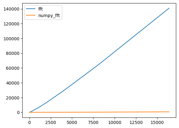
Pretty abysmal performance right? But numpy is done in C, and my lowly implementation is in python. I probably can do more speed up, but let’s compare it with the regular old DFT. Implementation bellow:
def DFT(X,inverse=False):
    RESULT = []
    N = len(X)
    sign =1
    if inverse:
        sign = -1
    for k in range(N):
        X_k = 0
        for n in range(N):
            X_k = X_k +  euler(N,sign*-k*n)*X[n]
        if inverse:
            RESULT.append(X_k/N)
        else:
            RESULT.append(X_k)
    return RESULT
Ok it’s a pretty simple algorithm and simple is always better right? Well let’s compare it.
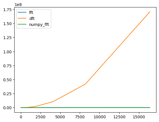
As we can see it absolutely dwarfs the FFT as the numbers increase. This is why FFT is such an important algorithm.
Footnotes
-
This has lit a fire inside me to create some sort of visual aid for these mathy blogs. I think if I am to make another blog on something similar, I will most definitely need it to communicate the concepts better. ↩